ARP protocol internals

ARP is a basic protocol in almost every TCP/IP implementation, but it normally does its work without the application or the system administrator being aware.  
    The ARP cache is fundamental to its operation, and we've used the arp(8) command to examine and manipulate the cache(The arp command displays and modifies entries in the ARP cache). Each entry in the cache has a timer that is used to remove both incomplete and completed(see below) entries.
    We followed through the normal operation of ARP along with specialized versions: proxy ARP (when a router answers ARP requests for hosts accessible on another of the router's interfaces) and gratuitous ARP (sending an ARP request for your own IP address, normally when bootstrapping). 

RFC 826 [Plummer 1982] is the specification of ARP.

Introduction

The problem that we deal with in this post is that IP addresses only make sense to the TCP/IP protocol suite. A data link such as an Ethernet or a token ring has its own addressing scheme (often 48-bit addresses) to which any network layer using the data link must conform.

A network such as an Ethernet can be used by different network layers at the same time. For example, a collection of hosts using TCP/IP and another collection of hosts using some PC network software can share the same physical cable.

When an Ethernet frame is sent from one host on a LAN to another, it is the 48-bit Ethernet address that determines for which interface the frame is destined.

The device driver software(in kernel) never looks at the destination IP address in the IP datagram.

Address resolution provides a mapping between the two different forms of addresses: 32-bit IP addresses and whatever type of address the data link uses.

Instead RARP (reverse address resolution protocol) is the ARP's (address resolution protocol) opposite.

RARP is used by systems without a disk drive (normally diskless workstations or X terminals) but requires manual configuration by the system administrator.

ARP provides a dynamic mapping from an IP address to the corresponding hardware address. The term dynamic mean it happens automatically and is normally not a concern of either the application user or the system administrator.

ARP's steps

 Whenever we type a command like:

$ ftp bsdi

the following steps take place as shown in Figure.

1. The application, the FTP client, calls the function gethostbyname(3) to convert the hostname (bsdi) into its 32-bit IP address. This function is called a resolver in the DNS (Domain Name System). This conversion is done using the DNS, or on smaller networks, a static hosts file (/etc/hosts).
2. The FTP client asks its TCP to establish a connection with that IP address.
3. TCP sends a connection request segment to the remote host by sending an IP datagram to its IP address.
4. If the destination host is on a locally attached network (e.g., Ethernet, token ring, or the other end of a point-to-point link), the IP datagram can be sent directly to that host. 
1. If the destination host is on a remote network, the IP routing function determines the Internet address of a locally attached next-hop router to send the IP datagram to. In either case the IP datagram is sent to a host or router on a locally attached network.
5. Assuming an Ethernet, the sending host must convert the 32-bit IP address into a 48-bit Ethernet address. A translation is required from the logical Internet address(IP) to its corresponding physical hardware address(MAC). This is the function of ARP.
1. ARP is intended for broadcast networks where many hosts or routers are connected to a single network.
6. ARP sends an Ethernet frame called an ARP request to every host on the network. This is called a broadcast. We show the broadcast in Figure upstairs with dashed lines. The ARP request contains the IP address of the destination host (whose name is bsdi) and is the request "if you are the owner of this IP address, please respond to me with your hardware address."
7. The destination host's ARP layer receives this broadcast, recognizes that the sender is asking for its hardware address, and replies with an ARP reply. 
1. This reply contains the IP address and the corresponding hardware address.
8. The ARP reply is received and the IP datagram that forced the ARP request-reply to be exchanged can now be sent.
9. The IP datagram is sent to the destination host.

The fundamental concept behind ARP is that the network interface has a hardware address (a 48-bit value for an Ethernet or token ring interface). Frames exchanged at the hardware level must be addressed to the correct interface. But TCP/IP works with its own 32-bit IP addresses.

Knowing a host's IP address doesn't let the kernel send a frame to that host. The kernel (i.e., the Ethernet driver) must know the destination's hardware address to send it data. The function of ARP is to provide a dynamic mapping between 32-bit IP addresses and the hardware addresses used by various network technologies.

Point-to-point links don't use ARP. When these links are configured (normally at bootstrap time) the kernel must be told of the IP address at each end of the link. Hardware addresses such as Ethernet addresses are not involved.

ARP Cache

Essential to the efficient operation of ARP is the maintenance of an ARP cache on each host. This cache maintains the recent mappings from Internet addresses to hardware addresses.

The normal expiration time of an entry in the cache is 20 minutes from the time the entry was created.

We can examine the ARP cache with the arp(8) command. The -a option displays all entries in the cache:

$ arp -a
sun (140.252.13.33) at 8:0:20:3:f6:42
svr4 (140.252.13.34) at 0:0:c0:c2:9b:26

The 48-bit Ethernet addresses are displayed as six hexadecimal numbers separated by colons.
 

ARP Packet Format

Figure below shows the format of an ARP request and an ARP reply packet, when used on an Ethernet to resolve an IP address. (ARP is general enough to be used on other networks and can resolve addresses other than IP addresses. The first four fields following the frame type field specify the types and sizes of the final four fields.). Look also here

• The first two fields in the Ethernet header are the source and destination Ethernet addresses.
• The special Ethernet destination address of all one bits means the broadcast address. All Ethernet interfaces on the cable receive these frames.
• The 2-byte Ethernet frame type specifies the type of data that follows. For an ARP request or an ARP reply, this field is 0×0806.
• The adjectives hardware and protocol are used to describe the fields in the ARP packets. 
• For example, an ARP request asks for the hardware address (an Ethernet address in this case) corresponding to a protocol address (an IP address in this case).
• The hard type field specifies the type of hardware address. 
• Its value is 1 for an Ethernet. 
• Prot type specifies the type of protocol address being mapped. 
• Its value is 0×0800 for IP addresses. This is purposely the same value as the type field of an Ethernet frame containing an IP datagram
• The next two 1-byte fields, hard size and prot size, specify the sizes in bytes of the hardware addresses and the protocol addresses. 
• For an ARP request or reply for an IP address on an Ethernet they are 6 and 4, respectively.
• The op field (This field is required since the frame type field is the same for an ARP request and an ARP reply ) specifies whether the operation is an 
• ARP request (a value of 1), 
• ARP reply (2), 
• RARP request (3), or 
• RARP reply (4)
• The next four fields that follow are(Notice there is some duplication of information: the sender's hardware address is available both in the Ethernet header and in the ARP request) 
• the sender's hardware address (an Ethernet address in this example), 
• the sender's protocol address (an IP address), 
• the target hardware address, and the 
• target protocol address
• For an ARP request all the fields are filled in except the target hardware address. 
• When a system receives an ARP request directed to it, it fills in its hardware address, swaps the two sender addresses with the two target addresses, sets the op field to 2, and sends the reply.

Proxy ARP

Proxy ARP lets a router answer ARP requests on one of its networks for a host on another of its networks. This fools the sender of the ARP request into thinking that the router is the destination host, when in fact the destination host is "on the other side" of the router. The router is acting as a proxy agent for the destination host, relaying packets to it from other hosts.

Figure 4.6 shows the arrangement, with a Telebit NetBlazer, named netb, between the subnet and the host sun.

When some other host on the subnet 140.252.1 (say, gemini) has an IP datagram to send to sun at address 140.252.1.29, gemini compares the network ID (140.252) and subnet ID (1) and since they are equal, issues an ARP request on the top Ethernet in Figure 4.6 for IP address 140.252.1.29. The router netb recognizes this IP address as one belonging to one of its dialup hosts, and responds with the hardware address of its Ethernet interface on the cable 140.252.1. The host gemini sends the IP datagram to netb across the Ethernet, and netb forwards the datagram to sun across the dialup SLIP link. This makes it transparent to all the hosts on the 140.252.1 subnet that host sun is really configured "behind" the router netb.

If we execute the arp command on the host gemini, after communicating with the host sun, we see that both IP addresses on the 140.252.1 subnet, netb and sun, map to the same hardware address. This is often a clue that proxy ARP is being used.    
  

$ arp -a
many lines for other hosts on the 140.252.1 subnet
netb (140.252.1.183) at 0:80:ad:3:6a:80
sun (140.252.1.29) at 0:80:ad:3:6a:80

Another detail in Figure 4.6 that we need to explain is the apparent lack of an IP address at the bottom of the router netb (the SLIP link). That is, why don't both ends of the dialup SLIP link have an IP address, as do both ends of the hardwired SLIP link between bsdi and slip? We noted in Section 3.8 that the destination address of the dialup SLIP link, as shown by the ifconfig command, was 140.252.1.183. The NetBlazer doesn't require an IP address for its end of each dialup SLIP link. (Doing so would use up more IP addresses.) Instead, it determines which dialup host is sending it packets by which serial interface the packet arrives on, so there's no need for each dialup host to use a unique IP address for its link to the router. All the dialup hosts use 140.252.1.183 as the destination address for their SLIP link.

Proxy ARP handles the delivery of datagrams to the router sun, but how are the other hosts on the subnet 140.252.13 handled? Routing must be used to direct datagrams to the other hosts. Specifically, routing table entries must be made somewhere on the 140.252 network that point all datagrams destined to either the subnet 140.252.13, or the specific hosts on that subnet, to the router netb. This router then knows how to get the datagrams to their final destination, by sending them through the router sun.

Proxy ARP is also called promiscuous ARP or the ARP hack. These names are from another use of proxy ARP: to hide two physical networks from each other, with a router between the two. In this case both physical networks can use the same network ID as long as the router in the middle is configured as a proxy ARP agent to respond to ARP requests on one network for a host on the other network. This technique has been used in the past to "hide" a group of hosts with older implementations of TCP/IP on a separate physical cable. Two common reasons for separating these older hosts are their inability to handle subnetting and their use of the older broadcasting address (a host ID of all zero bits, instead of the current standard of a host ID with all one bits).

Gratuitous ARP

Another feature of ARP that we can watch is called gratuitous ARP. It occurs when a host sends an ARP request looking for its own IP address. This is usually done when the interface is configured at bootstrap time.

In our internet, if we bootstrap the host bsdi and run tcpdump (We specified the -n flag for tcpdump to print numeric dotted-decimal addresses, instead of hostnames.) on the host sun, we see the packet shown below.

1  0.0  0:0:c0:6f:2d:40   ff:ff:ff:ff:ff:ff
arp who-has  140.252.13.35 tell 140.252.13.35

In terms of the fields in the ARP request, the sender's protocol address and the target's protocol address are identical: 140.252.13.35 for host bsdi. Also, the source address in the Ethernet header, 0:0:c0:6f:2d:40 as shown by tcpdump, equals the sender's hardware address.


Gratuitous ARP provides two features.

1. It lets a host determine if another host is already configured with the same IP address. The host bsdi is not expecting a reply to this request. But if a reply is received, the error message "duplicate IP address sent from Ethernet address: a:b:c:d:e:f" is logged on the console. This is a warning to the system administrator that one of the systems is misconfigured.
2. If the host sending the gratuitous ARP has just changed its hardware address (perhaps the host was shut down, the interface card replaced, and then the host was rebooted), this packet causes any other host on the cable that has an entry in its cache for the old hardware address to update its ARP cache entry accordingly. A little known fact of the ARP protocol [Plummer 1982] is that if a host receives an ARP request from an IP address that is already in the receiver's cache, then that cache entry is updated with the sender's hardware address (e.g., Ethernet address) from the ARP request. This is done for any ARP request received by the host. (Recall that ARP requests are broadcast, so this is done by all hosts on the network each time an ARP request is sent.)

[Bhide, Elnozahy, and Morgan 1991] describe an application that can use this feature of ARP to allow a backup file server to take over from a failed server by issuing a gratuitous ARP request with the backup's hardware address and the failed server's IP address. This causes all packets destined for the failed server to be sent to the backup instead, without the client applications being aware that the original server has failed.

Unfortunately the authors then decided against this approach, since it depends on the correct implementation of ARP on all types of clients. They obviously encountered client implementations that did not implement ARP according to its specification.

Monitoring all the systems on the author's subnet shows that SunOS 4.1.3 and 4.4BSD both issue gratuitous ARPs when bootstrapping, but SVR4 does not.

arp Command

We've used this command with the -a flag to display all the entries in the ARP cache.

The superuser can specify the -d option to delete an entry from the ARP cache.
Entries can also be added using the -s option. It requires a hostname and an Ethernet address: the IP address corresponding to the hostname, and the Ethernet address are added to the cache.

This entry is made permanent (i.e., it  won't time out from the cache) unless the keyword temp appears at the end of the command line.
The keyword pub at the end of a command line with the -s option causes the system to act as an ARP agent for that host. The system will answer ARP requests for the IP address corresponding to the hostname, replying with the specified Ethernet address. If the advertised address is the system's own, then this system is acting as a proxy ARP agent for the specified hostname.

ARP Examples

Here we'll use the tcpdump command to see what really happens with ARP when we execute normal TCP utilities such as Telnet.


Normal Example
To see the operation of ARP we'll execute the telnet command, connecting to the discard server.

$ arp -a     verify ARP cache is empty
$ telnet svr4 discard      connect to the discard server
Trying 140.252.13.34...
    Connected to svr4.
    Escape character is '^]'.
    ^]                              type Control, right bracket to get Telnet client prompt
    telnet> quit                    and terminate
    Connection closed.

While this is happening we run the tcpdump command on another system (sun) with the -e option(Print the link-level header on each dump line). This displays the hardware addresses (which in our examples are 48-bit Ethernet addresses).

We have deleted the final four lines of the tcpdump output that correspond to the termination of the connection, since they're not relevant to the discussion here.

1. In line 1 the hardware address of the source (bsdi) is 0:0:c0:6f:2d:40. The destination hardware address is ff:ff:ff:ff:ff:ff, which is the Ethernet broadcast address. Every Ethernet interface on the cable will receive the frame and process it.
2. The next output field on line 1, arp, means the frame type field is 0×0806, specifying either an ARP request or an ARP reply.
3. The value 60 printed after the words arp and ip on each of the five lines is the length of the Ethernet frame. 
1. Since the size of an ARP request and ARP reply is 42 bytes (28 bytes for the ARP message, 14 bytes for the Ethernet header), each frame has been padded to the Ethernet minimum: 60 bytes. This minimum of 60 bytes starts with and includes the 14-byte Ethernet header, but does not include the 4-byte Ethernet trailer. Some books state the minimum as 64 bytes, which includes the Ethernet trailer. We purposely did not include the 14-byte Ethernet header in the minimum of 46 bytes, since the corresponding maximum (1500 bytes) is what's referred to as the MTU maximum transmission unit. We use the MTU often, because it limits the size of an IP datagram, but are normally not concerned with the minimum. Most device drivers or interface cards automatically pad an Ethernet frame to the minimum size. The IP datagrams on lines 3, 4, and 5 (containing the TCP segments) are all smaller than the minimum, and have also been padded to 60 bytes.
4. The next field on line 1, arp who-has, identifies the frame as an ARP request with the IP address of svr4 as the target IP address and the IP address of bsdi as the sender IP address, tcpdump (by default) prints the hostnames corresponding to the IP address. (We'll use the -n option to see the actual IP addresses in an ARP request.)
5. From line 2 we see that while the ARP request is broadcast, the destination address of the ARP reply is bsdi (0:0:c0:6f:2d:40). The ARP reply is sent directly to the requesting host; it is not broadcast. tcpdump prints arp reply for this frame, along with the hostname and hardware address of the responder.
6. Line 3 is the first TCP segment requesting that a connection be established. Its destination hardware address is the destination host (svr4). 
7. The number printed after the line number on each line is the time (in seconds) when the packet was received by tcpdump. Each line other than the first also contains the time difference (in seconds) from the previous line, in parentheses. We can see in this figure that the time between sending the ARP request and receiving the ARP reply is 2.2 ms. The first TCP segment is sent 0.7 ms after this. The overhead involved in using ARP for dynamic address resolution in this example is less than 3 ms.
8. A final point from the tcpdump output is that we don't see an ARP request from svr4 before it sends its first TCP segment (line 4). 
1. While it's possible that svr4 already had an entry for bsdi in its ARP cache, normally when a system receives an ARP request addressed to it, in addition to sending the ARP reply it also saves the requestor's hardware address and IP address in its own ARP cache. This is on the logical assumption that if the requestor is about to send it an IP datagram, the receiver of the datagram will probably send a reply.

ARP Request to a Nonexistent Host
What happens if the host being queried for is down or nonexistent? To see this we specify a nonexistent Internet address the network ID and subnet ID are that of the local Ethernet, but there is no host with the specified host ID. From Figure 3.10 we see the host IDs 36 through 62 are nonexistent (the host ID of 63 is the broadcast address). We'll use the host ID 36 in this example.

bsdi# date ; telnet 140.252.13.36 ; date  telnet to an address this time, not a hostname
   Sat Jan 30 06:46:33 MST 1993
   Trying 140.252.13.36...
   telnet: Unable to connect to remote host: Connection timed out
   Sat Jan 30 06:47:49 MST 1993         76 seconds after previous date output
 bsdi# arp -a                        check the ARP cache
   ? (140.252.13.36) at (incomplete)

Figure 4.5 shows the tcpdump output.

This time we didn't specify the -e option since we already know that the ARP requests are broadcast.
What's interesting here is to see the frequency of the ARP requests: 5.5 seconds after the first request, then again 24 seconds later. (see TCP's timeout and retransmission algorithms) The total time shown in the tcpdump output is 29.5 seconds. But the output from the date commands before and after the telnet command shows that the connection request from the Telnet client appears to have given up after about 75 seconds. Indeed, most BSD implementations set a limit of 75 seconds for a TCP connection request to complete.

When we see the sequence of TCP segments that is sent to establish the connection, we'll see that these ARP requests correspond one-to-one with the initial TCP SYN (synchronize) segment that TCP is trying to send.
Note that on the wire we never see the TCP segments. All we can see are the ARP requests. Until an ARP reply comes back, the TCP segments can't be sent, since the destination hardware address isn't known. If we ran tcpdump in a filtering mode, looking only for TCP data, there would have been no output at all.


ARP Cache Timeout
A timeout is normally provided for entries in the ARP cache. (we'll see that the arp command allows an entry to be placed into the cache by the administrator that will never time out.)

Berkeley-derived implementations normally have a timeout of 20 minutes for a completed entry and 3 minutes for an incomplete entry. (We saw an incomplete entry in our previous example where we forced an ARP to a nonexistent host on the Ethernet.) These implementations normally restart the 20-minute timeout for an entry each time the entry is used.

The Host Requirements RFC says that this timeout should occur even if the entry is in use, but most Berkeley-derived implementations do not do this— they restart the timeout each time the entry is referenced.

Resources

TCP/IP Illustrated, Volume 1: The Protocols by W. Richard Stevens 
Attacks & Defences of the Data Link Layer

Computer Networks Performance

s

Network Performance

Up to this point (Computer Network Architecture ,   Computer Network Implementing Software), we have focused primarily on the functional aspects of networks. Like any computer system, however, computer networks are also expected to perform well, since the effectiveness of computations distributed over the network often depends directly on the efficiency with which the network delivers the computation’s data.

While the old programming adage “First get it right and then make it fast” is valid in many settings, in networking it is usually necessary to “design for performance.” 

It is therefore important to understand the various factors that impact network performance.

Bandwidth and Latency
Network performance is measured in two fundamental ways:

1. bandwidth (also called throughput) and 
2. latency (also called delay).

The bandwidth of a network is given by the number of bits that can be transmitted over the network in a certain period of time. 

For example, a network might have a bandwidth of 10 million bits/second (Mbps), meaning that it is able to deliver 10 million bits every second.

It is sometimes useful to think of bandwidth in terms of how long it takes to transmit each bit of data. On a 10-Mbps network, for example, it takes 1/10(Mbps)=0.1 microsecond (μs) to transmit each bit.

While you can talk about the bandwidth of the network as a whole, sometimes you want to be more precise, focusing, for example, on the bandwidth of a single physical link or of a logical process-to-process channel.

At the physical level, bandwidth is constantly improving, with no end in sight. 

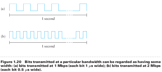
Intuitively, if you think of a second of time as a distance you could measure with a ruler, and bandwidth as how many bits fit in that distance, then you can think of each bit as a pulse of some width. For example, each bit on a 1-Mbps link is 1 μs wide, while each bit on a 2-Mbps link is 0.5 μs wide, as illustrated in Figure 1.20.

The more sophisticated the transmitting and receiving technology, the narrower each bit can become, and thus, the higher the bandwidth.

For logical process-to-process channels, bandwidth is also influenced by other factors, including how many times the software that implements the channel has to handle, and possibly transform, each bit of data.

The second performance metric, latency, corresponds to how long it takes a message to travel from one end of a network to the other. (As with bandwidth, we could be focused on the latency of a single link or an end-to-end channel.) Latency is measured strictly in terms of time. For example, a transcontinental network might have a latency of 24 milliseconds (ms); that is, it takes a message 24 ms to travel from one end of North America to the other.

There are many situations in which it is more important to know how long it takes to send a message from one end of a network to the other and back, rather than the one-way latency. We call this the round-trip time (RTT) of the network.

We often think of latency as having three components:

1. First, there is the speed-of-light propagation delay. This delay occurs because nothing, including a bit on a wire, can travel faster than the speed of light. If you know the distance between two points, you can calculate the speed-of-light latency, although you have to be careful because light travels across different mediums at different speeds: 
1. It travels at 3.0×10^8 m/s in a vacuum, 
2. 2.3×10^8 m/s in a cable, and 
3. 2.0×10^8 m/s in a fiber. 
2. Second, there is the amount of time it takes to transmit a unit of data. This is a function of the network bandwidth and the size of the packet in which
   the data is carried. 
3. Third, there may be queuing delays inside the network, since packet switches generally need to store packets for some time before forwarding them on an outbound link. 
4. So, we could define the total latency as:
1. Latency = Propagation + Transmit + Queue
2. Propagation = Distance/SpeedOfLight (where Distance is the length of the wire over which the data will travel, SpeedOfLight is the effective speed of light over that wire)
3. Transmit = Size/Bandwidth (Size is the size of the packet, andBandwidth is the bandwidth at which the packet is transmitted).

Note that if the message contains only one bit and we are talking about a single link (as opposed to a whole network), then the Transmit and Queue terms are not relevant, and latency corresponds to the propagation delay only.

Bandwidth and latency combine to define the performance characteristics of a given link or channel. Their relative importance, however, depends on the application.

For some applications, latency dominates bandwidth. For example, a client that sends a 1-byte message to a server and receives a 1-byte message in return is latency bound. Assuming that no serious computation is involved in preparing the response, the application will perform much differently on a transcontinental channel with a 100-ms RTT than it will on an across-the-room channel with a 1-ms RTT. Whether the channel is 1 Mbps or 100 Mbps is relatively insignificant, however, since the former implies that the time to transmit a byte (Transmit) is 8 μs and the latter implies Transmit = 0.08 μs.

In contrast, consider a digital library program that is being asked to fetch a 25-megabyte (MB) image—the more bandwidth that is available, the faster it will be able to return the image to the user. Here, the bandwidth of the channel dominates performance. To see this, suppose that the channel has  a bandwidth of 10 Mbps. It will take 20 seconds to transmit the image, making it relatively unimportant if the image is on the other side of a 1-ms channel or a 100-ms channel; the difference between a 20.001-second response time and a 20.1-second response time is negligible.

Figure 1.21 gives you a sense of how latency or bandwidth can dominate performance in different circumstances. The graph shows how long it takes to move objects  of various sizes (1 byte, 2 KB, 1 MB) across networks with RTTs ranging from 1 to 100 ms and link speeds of either 1.5 or 10 Mbps. We use logarithmic scales to show relative performance.

1. For a 1-byte object (say, a keystroke), latency remains almost exactly equal to the RTT, so that you cannot distinguish between a 1.5-Mbps network and a 10-Mbps network. 
2. For a 2-KB object (say, an email message), the link speed makes quite a difference on a 1-ms RTT network but a negligible difference on a 100-ms RTT network. 
3. And for a 1-MB object (say, a digital image), the RTT makes no difference—it is the link speed that dominates performance across the full range of RTT.

Note that we use the terms latency and delay in a generic way, that is, to denote how long it takes to perform a particular function such as delivering a message or moving an object. When we are referring to the specific amount of time it takes a signal to propagate from one end of a link to another, we use the term propagation delay. Also, we make it clear in the context of the discussion whether we are referring to the one-way latency or the round-trip time.

As an aside, computers are becoming so fast that when we connect them to networks, it is sometimes useful to think, at least figuratively, in terms of instructions per mile. Consider what happens when a computer that is able to execute 1 billion instructions per second sends a message out on a channel with a 100-ms RTT. (To make the math easier, assume that the message covers a distance of 5000 miles.) If that computer  sits idle the full 100 ms waiting for a reply message, then it has forfeited the ability to execute 100 million instructions, or 20,000 instructions per mile. It had better have been worth going over the network to justify this waste.

How Big Is a Mega?
There are several pitfalls you need to be aware of when working with the common units of networking—MB, Mbps, KB, and Kbps.

1. The first is to distinguish carefully between bits and bytes. Here, we always use a lowercase b for bits and a capital B for bytes. 
2. The second is to be sure you are using the appropriate definition of mega (M) and kilo (K). 
1. Mega, for example, can mean either 2^20 or 10^6 . 
2. Similarly, kilo can be either 2^10 or 10^3 . 

What is worse, in networking we typically use both definitions. Here’s why.  Network bandwidth, which is often specified in terms of Mbps is typically governed by the speed of the clock that paces the transmission of the bits. A clock that is running at 10 MHz is used to transmit bits at 10 Mbps. Because the
mega in MHz means 10^6 hertz, Mbps is usually also defined as 10^6 bits per second. (Similarly, Kbps is 10^3 bits per second.)

On the other hand, when we talk about a message that we want to transmit, we often give its size in kilobytes. Because messages are stored in the computer’s memory, and memory is typically measured in powers of two, the K in KB is usually taken to mean 2^10 . (Similarly, MB usually means 2^20 .) When you put
the two together, it is not un common to talk about sending a 32-KB message over a 10-Mbps channel, which should be interpreted to mean 32 × 2^10 × 8 bits are being transmitted at a rate of 10×10^6 bits per second. This is the interpretation we use here, unless explicitly stated otherwise.

The good news is that many times we are satisfied with a back-of-the-envelope calculation, in which case it is perfectly reasonable to pretend that a byte has 10 bits in it (making it easy to convert between bits and bytes) and that 10^6 is really equal to 2^20 (making it easy to convert between the two definitions of mega). Notice that the first approximation introduces a 20% error, while the latter introduces only a 5% error.

To help you in your quick-and-dirty calculations, 100 ms is a reasonable number to use for a cross-country round-trip time—at least when the country in question
is the United States—and 1 ms is a good approximation of an RTT across a local area network. In the case of the former, we increase the 48-ms round-trip time implied by the speed of light over a fiber to 100 ms because there are, as we have said, other sources of delay, such as the processing time in the switches inside the network. You can also be sure that the path taken by the fiber between two points will not be a straight line.

Delay × Bandwidth
It is also useful to talk about the product of these two metrics, often called the delay × bandwidth product. Intuitively, if we think of a channel between a pair of processes as a hollow pipe (see Figure 1.22), where

1. the latency corresponds to the length of the pipe and 
2. the bandwidth gives the diameter of the pipe, 
3. then the delay × bandwidth product gives the volume of the pipe—the number of bits it holds.

Said another way, if latency (measured in time) corresponds to the length of the pipe, then given the width of each bit (also measured in time), you can calculate how many bits fit in the pipe.

For example, a transcontinental channel with a one-way latency of 50 ms and a bandwidth of 45 Mbps is able to hold:

50 × 10^−3 seconds × 45 × 10^6 bits/second= 2.25 × 106 bits

or approximately 280 KB of data. In other words, this example channel (pipe) holds as many bytes as the memory of a personal computer from the early 1980s could hold.

The delay × bandwidth product is important to know when constructing high-performance networks because it corresponds to how many bits the sender must transmit before the first bit arrives at the receiver. 

If the sender is expecting the receiver to somehow signal that bits are starting to arrive, and it takes another channel latency for this signal to propagate back to the sender (i.e., we are interested in the channel’s RTT rather than just its one-way latency), then the sender can send up to two delay × bandwidth’s worth of data before hearing from the receiver that all is well. The bits in the pipe are said to be “in flight,” which means that if the receiver tells the sender to stop transmitting, it might receive up to a delay × bandwidth’s worth of data before the sender manages to respond.

In our example above, that amount corresponds to 5.5 × 106 bits (671 KB) of data. On the other hand, if the sender does not fill the pipe—send a whole delay × bandwidth product’s worth of data before it stops to wait for a signal—the sender will not fully utilize the network.
Note that most of the time we are interested in the RTT scenario, which we simply refer to as the delay × bandwidth product, without explicitly saying that this product is multiplied by two. Again, whether the “delay” in “delay × bandwidth” means one-way latency or RTT is made clear by the context.

High-Speed Networks
The bandwidths available on today’s networks are increasing at a dramatic rate, and there is eternal optimism that network bandwidth will continue to improve. This causes network designers to start thinking about what happens in the limit, or stated another way, what is the impact on network design of having infinite bandwidth available.

Although high-speed networks bring a dramatic change in the bandwidth available to applications, in many respects their impact on how we think about networking comes in what does not change as bandwidth increases: the speed of light. To quote Scotty from Star Trek, “You cannae change the laws of physics.”

In other words, “high speed” does not mean that latency improves at the same rate as bandwidth; 

the transcontinental RTT of a 1-Gbps link is the same 100 ms as it is for a 1-Mbps link.

To appreciate the significance of ever-increasing bandwidth in the face of fixed latency, consider what is required to transmit a 1-MB file over a 1-Mbps network versus over a 1-Gbps network, both of which have an RTT of 100 ms. In the case of the 1-Mbps network, it takes 80 round-trip times to transmit the file; during  each RTT, 1.25% of the file is sent. In contrast, the same 1-MB file doesn’t even come close to filling 1 RTT’s worth of the 1-Gbps link, which has a delay × bandwidth product of 12.5 MB. Figure 1.23 illustrates the difference between the two networks. In effect, the 1-MB file looks like a stream of data that needs to be transmitted across a 1-Mbps network, while it looks like a single packet on a 1-Gbps network. To help drive this point home, consider that a 1-MB file is to a 1-Gbps network what a 1-KB packet is to a 1-Mbps network.

Another way to think about the situation is that more data can be transmitted during each RTT on a high-speed network, so much so that a single RTT becomes a significant amount of time. Thus, while you wouldn’t think twice about the difference between a file transfer taking 101 RTTs rather than 100 RTTs (a relative difference of only 1%), suddenly the difference between 1 RTT and 2 RTTs is significant—a 100% increase.

In other words, latency, rather than throughput, starts to dominate our thinking about network design.

Perhaps the best way to understand the relationship between throughput and latency is to return to basics. The effective end-to-end throughput that can be achieved over a network is given by the simple relationship:

Throughput = TransferSize/TransferTime

where TransferTime includes not only the elements of one-way Latency identified earlier in this section, but also any additional time spent requesting or setting up the transfer.

Generally, we represent this relationship as:

TransferTime = RTT + 1/Bandwidth × TransferSize

We use RTT in this calculation to account for a request message being sent across the network and the data being sent back.

For example, consider a situation where a user wants to fetch a 1-MB file across a 1-Gbps network with a round-trip time of 100 ms. The TransferTime includes both the transmit time for 1 MB (1/1 Gbps × 1 MB = 8 ms), and the 100-ms RTT, for a total transfer time of 108 ms. This means that the effective throughput will be 1 MB/108 ms = 74.1 Mbps not 1 Gbps.

Clearly, transferring a larger amount of data will help improve the effective throughput, where in the limit, an infinitely large transfer size will cause the effective throughput to approach the network bandwidth. On the other hand, having to endure more than 1 RTT—for example, to retransmit missing packets—will hurt the effective throughput for any transfer of finite size and will be most noticeable for small transfers.

Application Performance Needs
The discussion in this section has taken a network-centric view of performance;  that is, we have talked in terms of what a given link or channel will support. The unstated assumption has been that application programs have simple needs—they want as much bandwidth as the network can provide. This is certainly true of the aforementioned digital library program that is retrieving a 25-MB image; the more bandwidth that is available, the faster the program will be able to return the image to the user.

However, some applications are able to state an upper limit on how much bandwidth they need. Video applications are a prime example. Suppose you want to stream a video image that is one-quarter the size of a standard TV image; that is, it has a resolution of 352 by 240 pixels. If each pixel is represented by 24 bits of information, as would be the case for 24-bit color, then the size of each frame would be (352 × 240 × 24)/8 = 247.5 KB
If the application needs to support a frame rate of 30 frames per second, then it might request a throughput rate of 75 Mbps. The ability of the network to provide more bandwidth is of no interest to such an application because it has only so much data to transmit in a given period of time.

Unfortunately, the situation is not as simple as this example suggests. Because the difference between any two adjacent frames in a video stream is often small, it is possible to compress the video by transmitting only the differences between adjacent frames. This compressed video does not flow at a constant rate, but varies with time according to factors such as the amount of action and detail in the picture and the compression algorithm being used. Therefore, it is possible to say what the average bandwidth requirement will be, but the instantaneous rate may be more or less.

The key issue is the time interval over which the average is computed. Suppose that this example video application can be compressed down to the point that it needs only 2 Mbps, on average. If it transmits 1 megabit in a 1-second interval and 3 megabits in the following 1-second interval, then over the 2-second interval it is transmitting at an average rate of 2 Mbps; however, this will be of little consolation to a channel that was engineered to support no more than 2 megabits in any one second. Clearly, just knowing the average bandwidth needs of an application will not always suffice.

Generally, however, it is possible to put an upper bound on how big of a burst an application like this is likely to transmit. A burst might be described by some peak rate that is maintained for some period of time. Alternatively, it could be described as the number of bytes that can be sent at the peak rate before reverting to the average rate or some lower rate. If this peak rate is higher than the available channel capacity, then the excess data will have to be buffered somewhere, to be transmitted later. Knowing how big of a burst might be sent allows the network designer to allocate sufficient buffer capacity to hold the burst.

Analogous to the way an application’s bandwidth needs can be something other than “all it can get,” an application’s delay requirements may be more complex than simply “as little delay as possible.” In the case of delay, it sometimes doesn’t matter so much whether the one-way latency of the network is 100 ms or 500 ms as how much the latency varies from packet to packet.

The variation in latency is called jitter.

Consider the situation in which the source sends a packet once every 33 ms, as would be the case for a video application transmitting frames 30 times a second.

• If the packets arrive at the destination spaced out exactly 33 ms apart, then we can deduce that the delay experienced by each packet in the network was exactly the same.
• If the spacing between when packets arrive at the destination—sometimes called the interpacket gap—is variable, however, then the delay experienced by the sequence of packets must have also been variable, and the network is said to have introduced jitter into the packet stream, as shown in Figure 1.24.

Such variation is generally not introduced in a single physical link, but it can happen when packets experience different queuing delays in a multihop packet-switched network. This queuing delay corresponds to the Queue component of latency defined earlier in this section, which varies with time.

To understand the relevance of jitter, suppose that the packets being transmitted over the network contain video frames, and in order to display these frames on the screen the receiver needs to receive a new one every 33 ms. If a frame arrives early, then it can simply be saved by the receiver until it is time to display it. Unfortunately, if a frame arrives late, then the receiver will not have the frame it needs in time to update the screen, and the video quality will suffer; it will not be smooth. Note that it is not necessary to eliminate jitter, only to know how bad it is. The reason for this is that if the receiver knows the upper and lower bounds on the latency that a packet can experience, it can delay the time at which it starts playing back the video (i.e., displays the first frame) long enough to ensure that in the future it will always have a frame to display when it needs it. The receiver delays the frame, effectively smoothing out the jitter, by storing it in a buffer.

Computer Network Implementing Software

f

Implementing Software

Network architectures and protocol specifications are essential things, but a good blueprint is not enough to explain the phenomenal success of the Internet: The number of computers connected to the Internet has been doubling every year since 1981 and is now approaching the impressive number of 1,966,514,816; It is believed that the number of bits transmitted over the Internet surpassed the corresponding figure for the voice phone system sometime in 2001.
What explains the success of the Internet?

1. There are certainly many contributing factors (including a good architecture), but 
2. one thing that has made the Internet such a runaway success is the fact that so much of its functionality is provided by software running in general-purpose computers. The significance of this is that new functionality can be added readily with “just a small matter of programming.” As a result, new applications and services—electronic commerce, videoconferencing, and packet telephony, to name a few—have been showing up at a phenomenal pace.
3. A related factor is the massive increase in computing power available in commodity machines. Although computer networks have always been capable in principle of transporting any kind of information, such as digital voice samples, digitized images, and so on, this potential was not particularly interesting if the computers sending and receiving that data were too slow to do anything useful with the information. Virtually all of today’s computers are capable of playing back digitized voice at full speed and can display video at a speed and resolution that is useful for some (but by no means all) applications. Thus, today’s networks have begun to support multimedia, and their support for it will only improve as computing hardware becomes faster.

The point to take away from this is that knowing how to implement network software is an essential part of understanding computer networks. With this in mind, this section first introduces some of the issues involved in implementing an application program on top of a network, and then goes on to identify the issues involved in implementing the protocols running within the network.

In many respects, network applications and network protocols are very similar—the way an application engages the services of the network is pretty much the same as the way a high-level protocol invokes the services of a low-level protocol. As we will see later in the section, however, there are a couple of important differences.

Application Programming Interface (Sockets)
The place to start when implementing a network application is the interface exported by the network.

Since most network protocols are implemented in software (especially those high in the protocol stack), and nearly all computer systems implement their network protocols as part of the operating system, when we refer to the interface “exported by the network,” we are generally referring to the interface that the OS provides to its networking subsystem. This interface is often called the network
application programming interface (API).

Although each operating system is free to define its own network API (and most
have), over time certain of these APIs have become widely supported; that is, they
have been ported to operating systems other than their native system. This is what has happened with the socket interface originally provided by the Berkeley distribution of Unix, which is now supported in virtually all popular operating systems.

The advantage of industry-wide support for a single API is that applications can be easily ported from one OS to another. 

It is important to keep in mind, however, that application programs typically interact with many parts of the OS other than the network; for example, they read and write files, fork concurrent processes, and output to the graphical display. Just because two systems support the same network API does not mean that their file system, process, or graphic interfaces are the same. Still, understanding a widely adopted API like Unix sockets gives us a good place to start.

Before describing the socket interface, it is important to keep two concerns separate in your mind.

1. Each protocol provides a certain set of services, and 
2. the API provides a syntax by which those services can be invoked in this particular OS. 
1. The implementation is then responsible for mapping the tangible set of operations and objects defined by the API onto the abstract set of services defined by the protocol. 
2. If you have done a good job of defining the interface, then it will be possible to use the syntax of the interface to invoke the services of many different protocols.
3. Such generality was certainly a goal of the socket interface, although it’s far from perfect.

The main abstraction of the socket interface, not surprisingly, is the socket. A good way to think of a socket is as the point where a local application process attaches to the network. The interface defines operations for

• creating a socket, 
• attaching the socket to the network, 
• sending/receiving messages through the socket, and 
• closing the socket. 

To simplify the discussion, we will limit ourselves to showing how sockets are used with TCP. The first step is to create a socket, which is done with the following operation:

int socket(int domain, int type, int protocol)

The reason that this operation takes three arguments is that the socket interface was designed to be general enough to support any underlying protocol suite. Specifically,

1. the domain argument specifies the protocol family that is going to be used: 
1. PF INET denotes the Internet family, 
2. PF UNIX denotes the Unix pipe facility, and 
3. PF PACKET denotes direct access to the network interface (i.e., it bypasses the TCP/IP protocol stack). 
2. The type argument indicates the semantics of the communication. 
1. SOCK STREAM is used to denote a byte stream. 
2. SOCK DGRAM is an alternative that denotes a message-oriented service, such as that provided by UDP. 
3. The protocol argument identifies the specific protocol that is going to be used. 
1. In our case, this argument is UNSPEC because the combination of PF INET and SOCK STREAM implies TCP. 
4. Finally, the return value from socket is a handle for the newly created socket, that is, an identifier by which we can refer to the socket in the future. 
1. It is given as an argument to subsequent operations on this socket.

The next step depends on whether you are a client or a server. On a server machine, the application process performs a passive open—the server says that it is prepared to accept connections, but it does not actually establish a connection. The server does this by invoking the following three operations:

int bind(int socket, struct sockaddr *address, int addr len)
int listen(int socket, int backlog)
int accept(int socket, struct sockaddr *address, int *addr len)

The bind operation, as its name suggests, binds the newly created socket to the specified address. This is the network address of the local participant—the server.

Note that, when used with the Internet protocols, address is a data structure that includes both the IP address of the server and a TCP port number. (As we know ports are used to indirectly identify processes. They are a form of demux keys as defined in an earlier post) 

The port number is usually some well-known number specific to the service being offered; for example, Web servers commonly accept connections on port 80.

The listen operation then defines how many connections can be pending on the specified socket. Finally, the accept operation carries out the passive open.

It is a blocking operation that does not return until a remote participant has established a connection, and when it does complete, it returns a new socket that corresponds to this just-established connection, and the address argument contains the remote participant’s address. 

Note that when accept returns, the original socket that was given as an argument still exists and still corresponds to the passive open; it is used in future invocations of accept.

On the client machine, the application process performs an active open; that is, it says who it wants to communicate with by invoking the following single operation:

int connect(int socket, struct sockaddr *address, int addr len)

This operation does not return until TCP has successfully established a connection, at which time the application is free to begin sending data. In this case, address contains the remote participant’s address. In practice, the client usually specifies only the remote participant’s address and lets the system fill in the local information.

Whereas a server usually listens for messages on a well-known port, a client typically does not care which port it uses for itself; the OS simply selects an unused one.

Once a connection is established, the application processes invoke the following two operations to send and receive data:

int send(int socket, char *message, int msg len, int flags)
int recv(int socket, char *buffer, int buf len, int flags)

The first operation sends the given message over the specified socket, while the second operation receives a message from the specified socket into the given buffer. Both operations take a set of flags that control certain details of the operation.

Example Application
We now show the implementation of a simple client/server program that uses the socket interface to send messages over a TCP connection. The program also uses other Unix networking utilities, which we introduce as we go. Our application allows a user on one machine to type in and send text to a user on another machine. It is a simplified version of the Unix talk program, which is similar to the program at the core of a Web chat room.

Client
We start with the client side, which takes the name of the remote machine as an argument.

1. It calls the Unix utility gethostbyname to translate this name into the remote host’s IP address. 
2. The next step is to construct the address data structure (sin) expected by the socket interface. Notice that this data structure specifies that we’ll be using the socket to connect to the Internet (AF INET). In our example, we use TCP port 5432 as the well-known server port; this happens to be a port that has not been assigned to any other Internet service. 
3. The final step in setting up the connection is to call socket and connect. Once the connect operation returns, the connection is established and the client program enters its main loop, which reads text from standard input and sends it over the socket.

#include <stdio.h>
#include <sys/types.h>
#include <sys/socket.h>
#include <netinet/in.h>
#include <netdb.h>

#define SERVER_PORT 5432
#define MAX_LINE 256
int main(int argc, char * argv[])
{
 FILE *fp;
 struct hostent *hp;
 struct sockaddr_in sin;
 char *host;
 char buf[MAX_LINE];
 int s;
 int len;
 if (argc==2) {
  host = argv[1];
 }
 else {
  fprintf(stderr, "usage: simplex-talk host\n");
  exit(1);
 }
 
/* translate host name into peer's IP address */
 hp = gethostbyname(host);
 if (!hp) {
  fprintf(stderr, "simplex-talk: unknown host: %s\n", host);
  exit(1);
 }
 
 /* build address data structure */
 bzero((char *)&sin, sizeof(sin));
 sin.sin_family = AF_INET;
 bcopy(hp->h_addr, (char *)&sin.sin_addr, hp->h_length);
 sin.sin_port = htons(SERVER_PORT);
 
 /* active open */
 if ((s = socket(PF_INET, SOCK_STREAM, 0)) < 0) {
  perror("simplex-talk: socket");
  exit(1);
 }
 if (connect(s, (struct sockaddr *)&sin, sizeof(sin)) < 0) {
  perror("simplex-talk: connect");
  close(s);
  exit(1);
 }
 
 /* main loop: get and send lines of text */
 while (fgets(buf, sizeof(buf), stdin)) {
  buf[MAX_LINE-1] = '\0';
  len = strlen(buf) + 1;
  send(s, buf, len, 0);
 }
}

Server The server is equally simple.

1. It first constructs the address data structure by filling in its own port number (SERVER PORT). By not specifying an IP address, the application program is willing to accept connections on any of the local host’s IP addresses. 
2. Next, the server performs the preliminary steps involved in a passive open: 
1. creates the socket, 
2. binds it to the local address, and 
3. sets the maximum number of pending connections to be allowed. 
4. Finally, the main loop waits for a remote host to try to connect, and 
5. when one does, receives and prints out the characters that arrive on the connection.  

#include <stdio.h>
#include <sys/types.h>
#include <sys/socket.h>
#include <netinet/in.h>
#include <netdb.h>

#define SERVER_PORT 5432
#define MAX_PENDING 5
#define MAX_LINE 256

int main()
{
 struct sockaddr_in sin;
 char buf[MAX_LINE];
 int len;
 int s, new_s;
 
 /* build address data structure */
 bzero((char *)&sin, sizeof(sin));
 sin.sin_family = AF_INET;
 sin.sin_addr.s_addr = INADDR_ANY;
 sin.sin_port = htons(SERVER_PORT);
 
 /* setup passive open */
 if ((s = socket(PF_INET, SOCK_STREAM, 0)) < 0) {
  perror("simplex-talk: socket");
  exit(1);
 }
 if ((bind(s, (struct sockaddr *)&sin, sizeof(sin))) < 0) {
  perror("simplex-talk: bind");
  exit(1);
 }
 listen(s, MAX_PENDING);
 
 /* wait for connection, then receive and print text */
 while(1) {
  if ((new_s = accept(s, (struct sockaddr *)&sin, &len)) < 0){
   perror("simplex-talk: accept");
   exit(1);
  }
  while (len = recv(new_s, buf, sizeof(buf), 0))
   fputs(buf, stdout);
  close(new_s);
 }
}

Protocol Implementation Issues
As mentioned at the beginning of this section, the way application programs interact with the underlying network is similar to the way a high-level protocol interacts with a low-level protocol. For example, TCP needs an interface to send outgoing messages to IP, and IP needs to be able to deliver incoming messages to TCP. This is exactly the service interface introduced in an earlier post.

Since we already have a network API (e.g., sockets), we might be tempted to use this same interface between every pair of protocols in the protocol stack. Although certainly an option, in practice the socket interface is not used in this way.

The reason is that there are inefficiencies built into the socket interface that protocol implementers are not willing to tolerate. Application programmers tolerate them because they simplify their programming task and because the inefficiency only has to be tolerated once, but protocol implementers are often obsessed with performance and must worry about getting a message through several layers of protocols. 

The rest of this section discusses the two primary differences between the network API and the protocol-to-protocol interface found lower in the protocol graph.

Process Model
Most operating systems provide an abstraction called a process, or alternatively, a thread.

Each process runs largely independently of other processes, and the OS is responsible for making sure that resources, such as address space and CPU cycles, are allocated to all the current processes. The process abstraction makes it fairly straightforward to have a lot of things executing concurrently on one machine; 

for example, each user application might execute in its own process, and various things inside the OS might execute as other processes. When the OS stops one process from executing on the CPU and starts up another one, we call the change a context switch.

When designing the network subsystem, one of the first questions to answer is, “Where are the processes?” There are essentially two choices, as illustrated in Figure 1.16.

1. In the first, which we call the process-per-protocol model, each protocol is implemented by a separate process. This means that as a message moves up or down the protocol stack, it is passed from one process/protocol to another—the process that implements protocol i processes the message, then passes it to protocol i − 1, and so on. 
1. How one process/protocol passes a message to the next process/protocol depends on the support the host OS provides for interprocess communication. 
1. Typically, there is a simple mechanism for enqueuing a message with a process. The important point, however, is that a context switch is required at each level of the protocol graph—typically a time-consuming operation.
2. The alternative, which we call the process-per-message model, treats each protocol as a static piece of code and associates the processes with the messages.
1. That is, when a message arrives from the network, the OS dispatches a process that it makes responsible for the message as it moves up the protocol graph. 
1. At each level, the procedure that implements that protocol is invoked, which eventually results in the procedure for the next protocol being invoked, and so on. 
2. For outbound messages, the application’s process invokes the necessary procedure calls until the message is delivered.

In both directions, the protocol graph is traversed in a sequence of procedure calls.

Although the process-per-protocol model is sometimes easier to think about—I implement my protocol in my process, and you implement your protocol in your process—the process-per-message model is generally more efficient for a simple reason: A procedure call is an order of magnitude more efficient than a context switch on most computers. The former model requires the expense of a context switch at each level,while the latter model costs only a procedure call per level.

Now think about the relationship between the service interface as defined above and the process model.

1. For an outgoing message, the high-level protocol invokes a send operation on the low-level protocol. Because the high-level protocol has the message in hand when it calls send, this operation can be easily implemented as a procedure call; no context switch is required. 
2. For incoming messages, however, the high-level protocol invokes the receive operation on the low-level protocol, and then must wait for a message to arrive at some unknown future time; this basically forces a context switch. 
1. In other words, the process running in the high-level protocol receives a message from the process running in the low-level protocol. This isn’t a big deal if only the application process receives messages from the network subsystem—in fact, it’s the right interface for the network API since application programs already have a process-centric view of the world—but it does have a significant impact on performance if such a context switch occurs at each layer of the protocol stack. It is for this reason that most protocol implementations replace the receive operation with a deliver operation. That is, the low-level protocol does an upcall—a procedure call up the protocol stack—to deliver the message to the high-level protocol.

Figure 1.17 shows the resulting interface between two adjacent protocols, TCP and IP in this case. In general, messages move down the protocol graph through a sequence of send operations, and up the protocol graph through a sequence of deliver operations.

Message Buffers
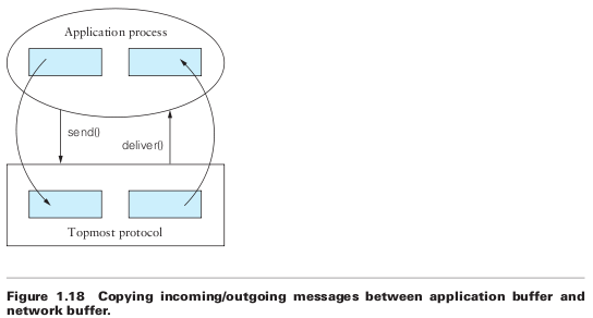
A second inefficiency of the socket interface is that the application process provides the buffer that contains the outbound message when calling send, and similarly it provides the buffer into which an incoming message is copied when invoking the receive operation. This forces the topmost protocol to copy the message from the application’s buffer into a network buffer, and vice versa, as shown in Figure 1.18.

It turns out that copying data from one buffer to another is one of the most expensive things a protocol implementation can do. This is because while processors are becoming faster at an incredible pace, memory is not getting faster as quickly as processors are.

Instead of copying message data from one buffer to another at each layer in the protocol stack, most network subsystems define an abstract data type for messages that is shared by all protocols in the protocol graph. Not only does this abstraction permit messages to be passed up and down the protocol graph without copying, but it usually provides copy-free ways of manipulating messages in other ways, such as adding and stripping headers, fragmenting large messages into a set of small messages, and reassembling a collection of small messages into a single large message. The exact form of this message abstraction differs from OS to OS, but it generally involves a linked list of pointers to message buffers, similar to the one shown in Figure 1.19.